The Variational Method
Interactive application and visualization of the variational method to aid conceptual understanding of introductory quantum mechanics, Arjan van der Vaart*, Sang T. Le Phan, and Brielle Wolfe, Department of Chemistry, University of South Florida, J. Chem. Educ. 102, 2160-2166 (2025).
This lab will introduce the linear variational method by calculating the ground state energy and wave function of a one-dimensional confined particle. These follow from the time-independent Schrödinger equation. The variational method solves this equation by expanding the unknown wave function as a linear combination of known functions, and subsequently minimizing the energy as a function of the unknown coefficients of this expansion.
1. Selection of the basis
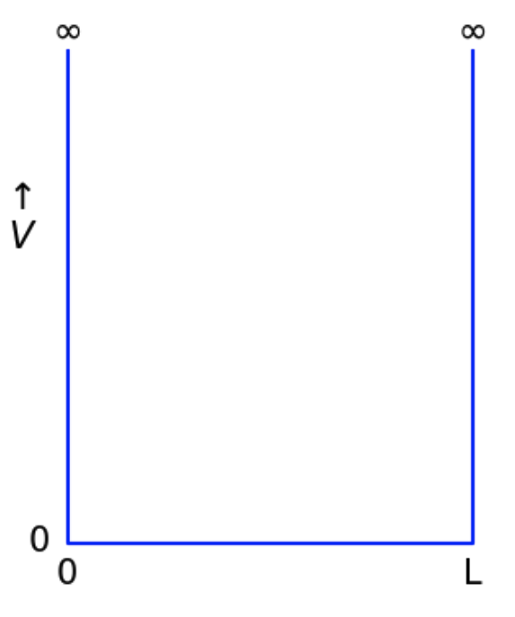
We aim to calculate the ground state energy ($E$) and wave function ($\Psi$) of a particle confined between $x=0$ and $L$ $\overset{\circ}{A}$ (where $1\,\overset{\circ}{A} = 10^{-10}$ m). The ground state is the lowest energy state and generally the most populated and important state. We will calculate these by solving the Schrödinger equation: $-\dfrac{\hbar^2}{2 m} \dfrac{d^2 \Psi(x)}{d x^2} + V(x) \Psi(x) = E\, \Psi(x)$. $E$ and $\Psi$ are the unknowns, $m$ is the mass of the particle, $\hbar$ is a constant, and $V(x)$ is the potential that acts on the confined particle. Since $E = K + V$, where $K$ is the kinetic energy, the term $-\dfrac{\hbar^2}{2 m} \dfrac{d^2}{d x^2}$ represents the kinetic energy: the higher the curvature of the wave function, the higher the kinetic energy. While the wave function itself is hard to interpret, its square $\vert \Psi(x) \vert^2 = \Psi^*(x) \Psi(x) = P(x)$ is the probability that the particle is at position $x$.
We proceed by expanding the wave function into a linear combination of $N$ known functions: $\Psi(x) = \sum\limits_{k=1}^N a_k \varphi_k(x)$, where $a_k$ are the unknown coefficients of the expansion. The $\varphi_k$ functions are called the basis functions, and collectively they form the basis set. What functions to pick? Since the particle is confined, its probability $P(0)=P(L)=0$; consequently $\Psi(0)=\Psi(L)=0$ (in fact, $P$ and $\Psi$ are zero for $x \notin (0, L)$). Therefore, we can simply choose functions $\varphi_k$ for which $\varphi_k(0) = \varphi_k(L) = 0$. A few possibilities:
"Legendre-like": $\;\varphi_k(x) = P_{2(k-1)+2}(\frac{2 x}{L}-1) - 1$ where $P_{j}$ is the $j^\text{th}$ Legendre polynomial. We only pick the even Legendre polynomials ($P_{2(k-1)+2}$), since the odd ones do not have the proper value at the $x=0$ and $x=L$ boundaries. We start from the 2$^\text{nd}$ Legendre polynomial since the zeroth would result in $\varphi=0$.
"Polynomial 1": $\;\varphi_k(x) = \left \{ \begin{array}{ll} x (x-L) & \text{if}\;k=1\\ x (x-L) (x-\frac{L}{2})^{k-1} & \text{if}\;k>1\end{array} \right .$
"Polynomial 2": $\;\varphi_k(x) = \left \{ \begin{array}{ll} x (x-L) & \text{if}\;k=1\\ x (x-L) \prod\limits_{i=1}^{k-1} (x-\frac{i L}{k}) & \text{if}\;k>1\end{array} \right .$
"Sin": $\;\varphi_k(x) = \sin(\frac{ k \pi x}{L})$
For simplicity, we restricted ourselves to real functions; therefore, $\Psi$ will also be real. Because of rounding errors, the maximum number of basis functions will be set differently for the "Sin" basis (50) than for the other bases (20).
Exercises Select "1. Show basis" for the Section button, deselect "Orthonormalize" and deselect "Calculate S".1a. Use the slider to set $L$ to 1.00 $\overset{\circ}{A}$. Visualize the various basis sets by pressing the red "Go" button, and verify that $\varphi_k(0)=\varphi_k(L)=0 \;\forall k$.
We can now derive how the ground state energy and wave function are obtained with the linear variational method. Introducing $\hat{H} = -\dfrac{\hbar^2}{2 m} \dfrac{d^2 }{d x^2} + V(x)$, we start by taking a generalized dot product of $\Psi$ with the Schrödinger equation. This gives $\int \Psi(x) \hat{H} \Psi(x) dx = E \int \Psi(x) \Psi(x) dx$, where we used the fact that by construction, our $\Psi$ is real. Since the particle is confined, $\Psi(x)=0$ for $x\notin (0, L)$, and the integration can be performed between $x=0$ and $L$.
The functional expansion of $\Psi$ over the $N$ real basis functions results in: $\int \Psi(x) \hat{H} \Psi(x) dx = \sum\limits_{i=1}^N \sum\limits_{j=1}^N a_i a_j \int \varphi_i(x)\hat{H}\varphi_j(x) dx = \sum\limits_{i=1}^N \sum\limits_{j=1}^N a_i a_j H_{ij}$, where $H_{ij} = \int \varphi_i(x) \hat{H} \varphi_j(x) dx$ is an element of the real, symmetric Hamiltonian matrix ($H$). Similarly, $\int \Psi(x) \Psi(x) dx = \sum\limits_{i=1}^N \sum\limits_{j=1}^N a_i a_j S_{ij}$, where $S_{ij} = \int \varphi_i(x) \varphi_j(x) dx$ is an element of the real, symmetric overlap matrix ($S$). Thus, we have translated the Schrödinger equation of our system to $\sum\limits_{i=1}^N \sum\limits_{j=1}^N a_i a_j H_{ij} = E \sum\limits_{i=1}^N \sum\limits_{j=1}^N a_i a_j S_{ij}$.
It would greatly help if the basis functions were orthonormal. To see this, let's use the notation $\phi_k$ for orthonormal basis functions. If the basis functions were orthonormal, then $S_{ij} = \int \phi_i(x) \phi_j(x) dx = \left \{ \begin{array}{ll}0 & \text{if}\;i\ne j\\1 & \text{if}\;i = j\end{array}\right .$. Then: $\sum\limits_{i=1}^N \sum\limits_{j=1}^N a_i a_j H_{ij} = E \sum\limits_{i=1}^N \sum\limits_{j=1}^N a_i a_j S_{ij} = E \sum\limits_{i=1}^N a_i^2$. Differentiating this equation to $a_k$ gives $2 \sum\limits_{i=1}^N a_k H_{ik} = \dfrac{\partial E}{\partial a_k}\sum\limits_{i=1}^N a_i^2 + 2 E a_k$, where we used the fact that $H$ is symmetric. In the ground state, the energy is minimal, or $\dfrac{\partial E}{\partial a_k}=0\;\forall k$. Therefore, $\sum\limits_{i=1}^N a_k H_{ik} = E a_k$, or $H \overrightarrow{a} = E \overrightarrow{a}$, where $\overrightarrow{a}$ is the vector of $a_k$ coefficients.
In other words, $E$ is an eigenvalue of the $H$ matrix, and $\overrightarrow{a}$ the associated normalized eigenvector. Both will be real, since the $H$ matrix is real and symmetric. The wave function is obtained from $\Psi(x) = \sum a_k \phi_k(x)$, or the dot product of $\overrightarrow{a}$ with the basis. The components of this eigenvector represent the relative weight/importance of the basis functions: if $a_i = 0$, the weight of $\phi_k$ is $0$, and $\phi_k$ does not contribute to the wave function. Since the ground state is the lowest energy state, the ground state energy is the lowest eigenvalue, and the ground state wave function its associated eigenvector. We will use subscript "0" for all ground state properties (e.g. $E_0$, $\Psi_0$, and $P_0$).
In conclusion, by selecting orthonormal basis functions $\phi_k$, the ground state energy ($E_0$) is the lowest eigenvalue of the $H$ matrix and the wave function ($\Psi_0$) is obtained from the dot product of the associated eigenvector $\overrightarrow{a}$ with the basis. The $i^\text{th}$ component of the eigenvector ($a_i$) indicates the weight of the $i^\text{th}$ basis function ($\phi_i$).
Exercises Select "1. Show basis" for the Section button and deselect "Orthonormalize".1d. Using $N=5$, now select "Calculate S" to evaluate the overlap matrix and check if our bases are orthonormal. Because computers represent numbers using finite precision, tiny numbers like -6.47e-16 $=-6.47\cdot 10^{-16}$ and 3.78e-14 $=3.78\cdot 10^{-14}$ can safely be interpreted as zero.
Clearly, none of our bases is orthonormal, and only the "Sin" basis is orthogonal. Happily, we can readily orthogonalize and normalize our bases by using the Gram-Schmidt procedure.
Exercises Select "1. Show basis" for the Section button.1e. Orthonormalize the bases by selecting "Orthonormalize". Use $N=5$ to examine how the orthonormal $\phi_k$ functions differ from the original $\varphi_k$ basis.
We're ready to use the variational method for several systems (Sections 2-6). All bases will automatically be orthonormalized in the next sections. Each application will result in 3 graphs:
Left graph. This shows the grounds state wave function ($\Psi_0(x)$) in black with values on the left $y$-axis. The potential $V(x)$ within the confined space is shown in bright blue with values (in eV) on the right $y$-axis; these values are identical to values on the right $y$-axis of the middle graph.
Middle graph. The ground state probability that the electron is at position $x$ is shown as a black curve. This probability equals $P_0(x)=\vert \Psi_0(x)\vert^2$, values are reported on the left $y$-axis. The light blue shading underneath this curve represents the ground state probability that the electron is between $x_{-}$ and $x_{+}$; this probability equals $\int_{x_{-}}^{x_{+}} P_0(x) dx$. The value of this probability is printed underneath the graph; $x_{-}$ and $x_{+}$ are set by a slider. The bright blue curve shows the potential $V(x)$ within the confined space; values (in eV) are reported on the right $y$-axis. This potential is also shown in bright blue in the left graph.
The top of this graph reports the ground state energy ($E_0$), as well as the ground state kinetic ($K_0 = -\frac{\hbar^2}{2 m}\int \Psi_0(x) \frac{d^2 \Psi_0(x)}{d x^2} dx$) and potential ($V_0 = \int \Psi_0(x) V(x) \Psi_0(x) dx$) energies (in eV); $\;E_0 = K_0 + V_0$. To clarify: $V(x)$ is the external potential, the potential felt by the particle, while $V_0$ is the potential energy of the particle in the ground state. As the expression suggests, the kinetic energy is closely related to the curvature of the wave function: no curvature, no kinetic energy, and high curvature, high kinetic energy.
Right graph. This graph shows the $a_k$ values of the ground state eigenvector. These can be interpreted as the weights of the basis functions $\phi_k$ for the ground state wave function: zero $a_k$, means zero weight for $\phi_k$. In order words, if $a_k=0$ then $\phi_k$ has no contribution to $\Psi_0$.
Energies, probabilities, and first few $a_k$ elements are also printed underneath the graphs; you can use the mouse to copy these.
2. Particle in a box
We will first consider a particle in a box: a confined system for which $V(x)=0$:
2a. Using the mouse to copy and paste, complete the following table with reported total ground state energies $E_0$ (in eV), using all decimals:
| N | Legendre-like | Polynomial 1 | Polynomial 2 | Sin |
|---|---|---|---|---|
| 1 | ||||
| 2 | ||||
| 3 | ||||
| 4 | ||||
| 5 |
Use this filled-out table to answer the next questions.
The behavior of Exercise 2e can be explained by symmetry. $V(x)$ is symmetric with respect to a reflection at $x=\frac{L}{2}$. Our wave function has to obey the same symmetry: if the potential is symmetric upon reflection, our ground state wave function has to be symmetric upon reflection as well. This symmetry upon reflection is called parity; parity is even for symmetry and odd for antisymmetry upon reflection. We will encounter the effect of parity many times.
2f. Examine which of the "Polynomial 1"/"Polynomial 2" $\phi_k$ basis functions are symmetric upon reflection, and use this to explain your observations of Exercise 2e.Why do symmetric potentials give even parity ground state wave functions? First consider the wave function for any energy state (not just the ground state). The probability should be symmetric when the potential is symmetric (because the particle feels the same on either side of the midpoint). The probability is the square of the wavefunction, so the wave function is either symmetric or antisymmetric for symmetric potentials. Now, let's apply this finding to the ground state. The ground state has the lowest energy ($E$). The lower the curvature of the wave function, the lower the kinetic energy ($K$), and therefore the lower the total energy ($E=K+V$). Thus, the fewer nodes (places where the wave function equals zero) the wave function has, the lower the curvature, and the lower the energy; in fact, the lowest energy wave function will have no nodes. No nodes is only possible for a wave function with even parity. This proves that symmetric potentials will have even parity ground states.
2g. Use the left graph to verify that the ground state wave function has even parity for all bases and no nodes.Since the ground state wave function doesn't have nodes, the ground state probability distribution ($P_0(x)$) won't either. Thus, the ground state will be maximally delocalized (spread out over space). The more delocalized the system, the lower the energy.
2h. In words, explain why the ground state is maximally delocalized.
The variational method obtained the ground state by minimizing the energy. This was shown to correspond to solving the eigenvalue equation $H \overrightarrow{a} = E \overrightarrow{a}$. The ground state energy ($E_0$) is then the lowest eigenvalue, with the ground state wave function ($\Psi_0$) the associated eigenvector. But what are the other eigenvalues/eigenvectors?
The other eigenvalues are the energies of the excited states, and the associated eigenvectors the wave functions of the excited states. Excited states are states that are higher in energy; these play important roles in photochemistry, for example. In general, the variational method is less good at calculating excited states. It gives an upper bound for these states, but deviations with the "true" excited states are generally larger than for the "true" ground states. We can show this deficiency for the particle in the box when using the "Legendre-like" basis (exercise 2k). In contrast, the "Sin" base will give the exact value of the excited states of the particle in a box, since the "Sin" base yields the exact analytical solution for this problem (see exercise 2h).
2k. Visualize the excited states of the particle in a box by selecting the "Sin" basis and selecting "Show excited states". The left graph shows the energy of the excited states as a straight line; the the shape of the associated wave function is also shown. The ground state is shown in black, the potential in bright blue. How many nodes does the ground state, the first excited state, the second excited state, the third excited state, ...., have?2l. What state is the most delocalized?
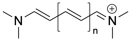
The length of the conjugated chain backbone is $2.49 (n + 1) + 5.67\;\overset{\circ}{A}$. $\pi$-electrons will occupy energy levels in pairs, starting from the lowest energy level. The highest occupied energy level is called the HOMO, the lowest unoccupied energy level the LUMO. Thus, for the $n=0$ cyanine dye, the HOMO is the third energy level (or second excited state above the ground state), the LUMO the fourth (or third excited state). The transition from the HOMO to the LUMO can be measured with UV-vis spectroscopy; the wave length of the transition follows from $E_{LUMO}-E_{HOMO}=h \nu = \frac{h c}{\lambda}$, where $\nu$ is the frequency, $\lambda$ the wave length, $c$ the speed of light ($c=299792458$ m/s), and $h$ the Planck constant ($h=6.62607015\cdot 10^{-34}$ J$\cdot$s). Using the particle in a box model for $E_{HOMO}$ and $E_{LUMO}$, calculate the wave length of the HOMO to LUMO transition for cyanine dyes with $n=0$, $n=1$, and $n=2$; 1 eV = $1.602176634\cdot 10^{-19}$ J. What colors do these wave lengths correspond to? Experimentally, the transitions are found at 313, 416, and 519 nm, respectively.
3. Step potential
Let's now consider $V(x)\ne 0$; unlike the particle in a box potential, $V(x)\ne 0$ does not have an exact analytical solution. The sliders implement:
$V(x) = \left \{ \begin{array}{ll}V(x) = 0 & \text{if} \; x< x_{1}\\ V(x) = h_1 & \text{otherwise}\end{array} \right .$
We now have two regions: a region where $V(x)=0$ eV and a region where $V(x)=h_1$ eV. Unlike the particle in a box, the potential is not symmetrical; consequences of this will be encountered in the exercises below. We expect a difference in probabilities over these regions, since particles prefer regions of low potential.
Exercises Select "3. Step potential" for the Section button, deselect "Show excited states", choose "Electron" for mass, and set $L$ to $1.00\;\overset{\circ}{A}$. Set $x_1=0.5\;\overset{\circ}{A}$ and $h_1$ to 100 eV. Set $x_{-}-x_{+}$ (for $P_0$) to 0.5-1.0.3a. Use the "Sin" basis to compare the shape of $P_0(x)$ and the total probability between $x=0.5$ and $x=1.0$ (the value of $\int\limits_{0.5}^{1.0} P_0(x) dx$, which is printed below the graph and shaded light blue in the graph) when $N=1$ and when $N=2$. Explain the difference.
Tunneling is favorable, since it allows the system to spread out more (become more delocalized; see Exercise 2h and 2j): it can spread out over into the classically forbidden barrier region. We can also show favorability of tunneling by comparing the energy of a step potential to that of a particle in a box. When $L$ is identical, the particle in a box is favored (has lower energy):
But when we compare a step potential in a box of length $L$ to a particle in a box of length $x_1$, the favorable energetic effect of tunneling is clearly visible:
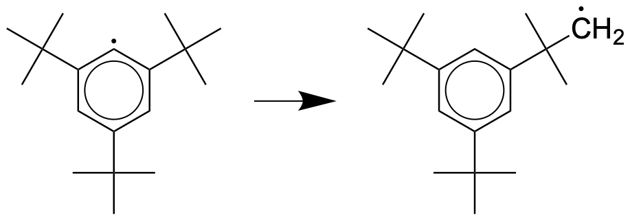
3f. Use the "Sin" basis and $N=50$ to compare the ground state energy for the step potential with $L=2$, $x_1=1$ and $h_1=5000$, to that of the particle in a box with $L=1$. Was there tunneling in the step potential? Based on this comparison, is tunneling energetically favorable?Exercise 3g shows that tunneling strongly depends on mass: light particles tunnel more easily than heavy particles. In chemistry tunneling is responsible for very large kinetic isotope effects: the observation that certain reactions involving hydrogen atoms are much faster than the same reaction done with deuterons (heavy hydrogen). Tunneling is also responsible for the very high rates of certain reactions, for example the intramolecular rearrangement of aryl radicals such as 2,4,6-tri-tert-butylphenyl to 3,5-di-tertbutylneophyl:
We will see another important example of tunneling in chemistry in exercise 6c-e.
4. Central potential
For the central potential: $V(x) = \left \{ \begin{array}{ll}0 & \text{if} \; x< x_{11}\\ h_1 & \text{if} \; x_{11} \le x \le x_{12}\\ 0 & \text{if} \; x> x_{12}\end{array} \right .$
Exercises. Select the "4. Central potential" section. Set $L=1$ and set the $x_{11}-x_{12}$ sliders to 0.3-0.7. Set $x_{-}-x_{+}$ to 0.3-0.7. Deselect "Show excited states", choose "Electron" for mass.4a. Use the "Sin" basis with $N=50$ to compare the value of the total probabililty between $x=0.3$ and $x=0.7$ (i.e. $\int\limits_{0.3}^{0.7} P_0(x) dx$) when $h_1=0$ and $h_1=10$. Explain the difference.
4b. Use the "Sin" basis, $N=50$, and $h_1=150$. What are the values of $E_0$ and $\int\limits_{0.3}^{0.7} P_0(x) dx$? Would $\int\limits_{0.3}^{0.7} P_0(x) dx>0$ for a classical system? What is this quantum mechanical behavior called?
5. Double barrier potential
For the double barrier potential: $V(x) = \left \{\begin{array}{ll} h_1 & \text{if} \; x_{11} \le x \le x_{12}\\ h_2 & \text{if} \; x_{21} \le x \le x_{22}\\ 0 & \text{otherwise}\end{array} \right .$
Exercises. Select the "5. Double barrier potential" section. Set $L=2$, $x_{11}-x_{12}$ to 0.4-0.8, and $x_{21}-x_{22}$ to 1.2-1.6; set $x_{-}-x_{+}$ to 0.8-1.2. Deselect "Show excited states", choose "Electron" for mass.5a. Set $h_1$ and $h_2$ to 50, and investigate which basis is the best. Do this for $N\le 20$.
6. Intersecting parabolas
Covalent bonds can be approximated as a spring. The potential for a spring is parabolic: $V(x)=k_1 (x-x_1)^2$, where $k_1$ is the force constant, $x$ the length of the spring, and $x_1$ the resting/equilibrium length of the spring. This spring model is called "the harmonic oscillator" and describes bond vibrations.
Exercises. Let's first model the proton in hydrogen chloride, HCl. Select "6. Intersecting parabola" for section. Select "proton" for mass. Set $L$ to 2.0, $h_2$ to 4000, $x_1$ to 1.0 and $x_2$ to 2.0. Set $k_1$ to 16.2, set $k_2$ to 500. Select the "Sin" base, and set $N$ to 50. Set $x_{-}-x_{+}$ to 0.8-1.2. Select "Show excited states"; while the variational method generally converges more poorly for excited states, it works well for the first 5 excited states of the problems presented here.6a. How are the energy levels spaced apart? Does this type of spacing differ from that of the particle in a box?
Ammonia (NH$_3$) is a pyramidal (umbrella shaped) molecule. Like an umbrella in the wind, it can undergo an inversion, turning the molecule "inside out". This process is depicted in the following potential energy diagram:
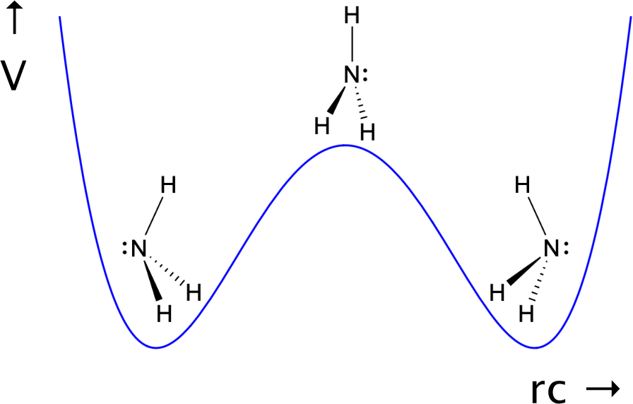
A good reaction coordinate coordinate (i.e. a geometrical function that describes the chemical change) is the position of the nitrogen atom. It switches place from left to right, and vice-versa, moving about 0.8 $\overset{\circ}{A}$ in the process. The stable "left" and "right" conformations are energy wells, that resemble parabola; in the stable conformations, nitrogen vibrates around the energy minima of the wells. The wells are separated by an energy barrier, which needs to be overcome for inversion. The transition state ($\ddagger$, the highest energy intermediate) is a planar molecule; this state is 0.2508 eV above the stable conformations.
6c. Calculate the rate of ammonia inversion at room temperature with classical transition state theory: $ k = \frac{k_B T}{h}e^{-\Delta G^\ddagger/(k_B T)}$, where $k_B$ is the Boltzmann constant ($k_B = 1.380649\cdot10^{-23}$ J/K), $h$ the Planck constant ($h=6.62607015\cdot 10^{-34}$ J$\cdot$s), and 1 eV = $1.602176634\cdot 10^{-19}$ J. Since the entropic contribution is small, you can use $\Delta G^\ddagger \approx \Delta E^\ddagger$.Even when performing the classical calculation correctly (taking the small entropic contribution into account), the calculated rate is about 100 times less than the experimentally measured rate of $4.74\cdot 10^{10}$ s$^{-1}$. The difference is due to tunneling: by penetrating the barrier, the crossing rate is significantly increased.
6d. Let's calculate this rate by considering the energy levels of ammonia. The inversion potential is modeled by $V(x)=\frac{k(x^2-r^2)^2}{8 r^2}$, and hard-coded in the "6d. Ammonia inversion" section. This setting uses the proper mass and the "Sin" basis set with $N=50$; while the variational method generally converges more poorly for excited states, it works well for the first few excited states shown here. The energy of the barrier is printed below the graphs.Calculate the ground state and first 5 excited states for the inversion of ammonia, and describe what this energy diagram looks like.
Intersecting parabolas can serve as a simplistic model for reactions where a bond is broken and formed (say, the $A \rightleftarrows B$ reaction):
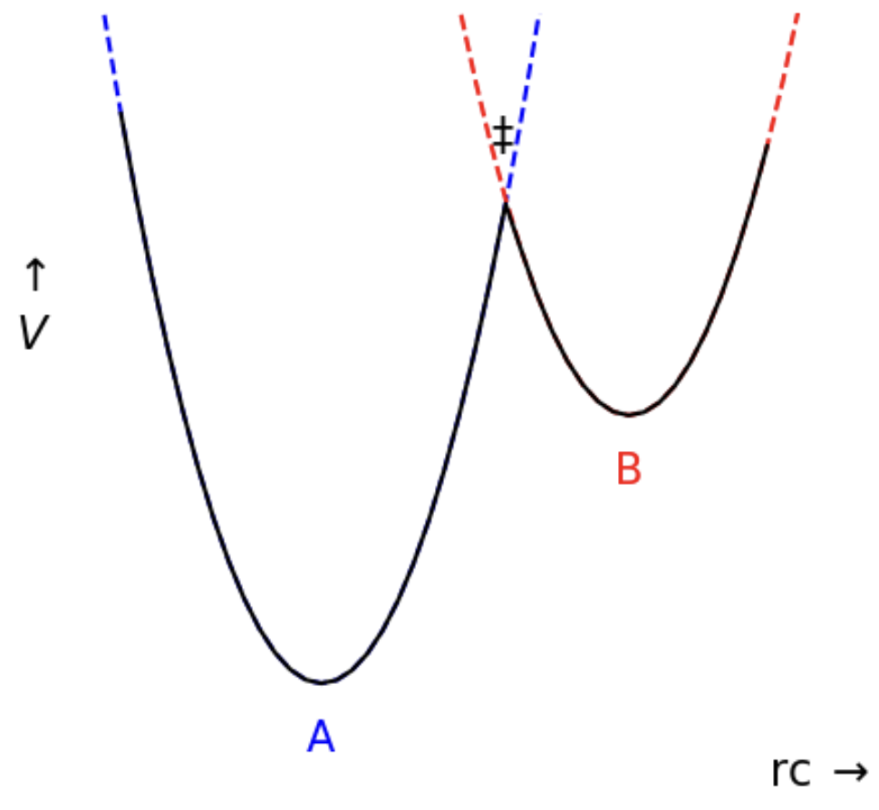
$A$ and $B$ are stable compounds, described by energy wells. In the simplest form, these are given by parabolas (blue for $A$ and red for $B$). The reaction will follow the lowest energy path (black). The transition state ($\ddagger$) is where the two parabolas cross; this is the highest energy intermediate in the reaction. Our description is not only simplistic; it also misses temperature effects.
Exercises. Let's model a proton transfer reaction. Select "6. Intersecting parabola" for section. Set $L=2$, $N=20$. Set $h_2=0.15$, $k_1=16$, $k_2=16$, $x_1=0.5$, and $x_2=1.5$. Set mass to "Proton"; deselect "Show excited states". Output will now include the position of the crossing point (i.e. the position of $\ddagger$) and its energy, and the probability between $x=0$ and the crossing point ($P_A$). $P_A$ corresponds to the probability to be in the $A$ well: the probability to be compound $A$. $P_B = 1-P_A$: this is the probability to be in the $B$ well, or the probability to be compound $B$.Exercise 6f. Compare the energy and probability distribution of the "Sin" basis to that of the "Legendre-like" basis. Why is the "Legendre-like" basis so bad?
As exercise 6g showed, the difference in basin energy is a determining factor if $A$ or $B$ is favored (more probable). Another important factor is the curvature of the basins. The final exercise shows an extreme case: